The objective of this design project was to produce a low-battery level detector. The low-battery circuit is powered by a 3.7 V lithium ion battery with a graphite anode. The specifications (both mandatory and optional) for a working design are as followed:
Mandatory
The battery can’t be allowed to decrease below 2.4 V, or an internal chemical reaction will occur. This reaction will cause one of the battery electrodes to oxidize/corrode through a process which can’t be reversed through recharging. Thus, the battery capacity will be lost and the cell may be completely destroyed.
Li-Ion cells will not tolerate trickle charging (charging a fully charged battery at a rate equal to its self-discharge rate, thus enabling the battery to remain at its fully charged level) after they are fully charged. Even if a small amount of current is continuously forced into a fully-charged Li-Ion cell, the cell will be damaged. So this means that Li-Ion cells should be charged using constant-voltage (C-V) chargers, and not constant-current (C-C) chargers.
Batteries are acutely sensitive to operating temperature with respect to their charging characteristics and A-hr capacity. Most well-designed chargers have temperature sensors to assure that the battery temperature is within the allowable “window” for charging (if not, the charger will not turn on the current source). The Li-Ion cell can be safely charged at temperatures between 0 - 45°C. The operating temperature range during discharge is specified as -20 to 60°C.
The design of the Low-battery level indicator consisted of the lithium ion battery and the voltage comparator.
According to Figure 1, the build of a lithium ion battery was required to match the decaying curve of the graphite anode.
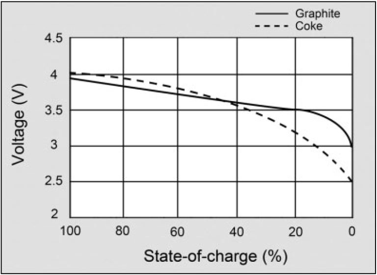
Figure 1: Low-battery circuit with 3.7 V lithium ion battery
Within the Synopsis design tool, the Galaxy Custom Designer was implemented to perform this function and many others.
In Figure 2, the 3.7 V lithium ion battery was constructed with a "VPWL" (Piecewise-Linear voltage source) cell,
which consisted of 22 time value pairs. The time value pairs are displayed in Table 1. These pairs display the actual linear and exponential decay.
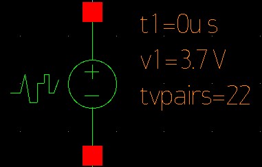
Figure 2: 3.7 V Lithium Ion battery as it appears in all schematics
| Time 1 = 0 µs | Voltage 1 = 3.7 V |
|---|---|
| Time 2 = 80 µs | Voltage 2 = 3.5 V |
| Time 3 = 81 µs | Voltage 3 = 3.5 V |
| Time 4 = 82 µs | Voltage 4 = 3.49 V |
| Time 5 = 83 µs | Voltage 5 = 3.49 V |
| Time 6 = 84 µs | Voltage 6 = 3.48 V |
| Time 7 = 85 µs | Voltage 7 = 3.48 V |
| Time 8 = 86 µs | Voltage 8 = 3.47 V |
| Time 9 = 87 µs | Voltage 9 = 3.46 V |
| Time 10 = 88 µs | Voltage 10 = 3.45 V |
| Time 11 = 89 µs | Voltage 11 = 3.43 V |
| Time 12 = 90 µs | Voltage 12 = 3.41 V |
| Time 13 = 91 µs | Voltage 13 = 3.38 V |
| Time 14 = 92 µs | Voltage 14 = 3.35 V |
| Time 15 = 93 µs | Voltage 15 = 3.31 V |
| Time 16 = 94 µs | Voltage 16 = 3.25 V |
| Time 17 = 95 µs | Voltage 17 = 3.18 V |
| Time 18 = 96 µs | Voltage 18 = 3.10 V |
| Time 19 = 97 µs | Voltage 19 = 3.01 V |
| Time 20 = 98 µs | Voltage 20 = 2.92 V |
| Time 21 = 99 µs | Voltage 21 = 2.83 V |
| Time 22 = 100 µs | Voltage 22 = 2.74 V |
Table 1: Time Value Pairs for VBat
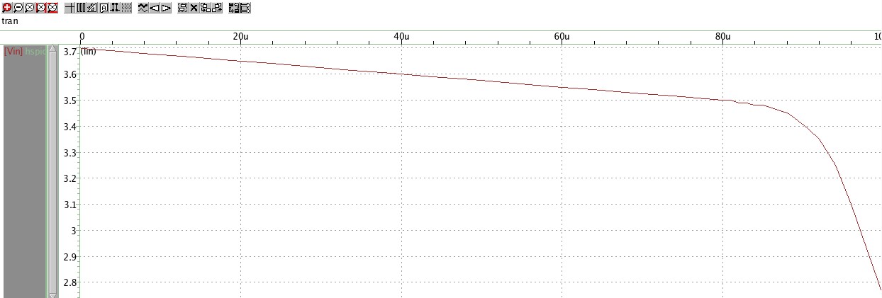
Figure 3: Transient Analysis of Lithium Ion Battery Simulation
After the battery was built, output pins were attached and a transient analysis was simulated to ensure its correctness of behavior, as its decay was not strictly linear. The simulation of the battery can be viewed in Figure 3. At a 100% state of charge, the battery is charged at 3.7 V. From 100% to 20%, the battery’s voltage decreases linearly from 3.7 V to 3.5 V. From 20% to 0%, the battery’s voltage has an exponential decay from 3.5 V to 3 V. This output behavior can be used for signaling a battery’s imminent failure by connecting a resistor with a value of 105 to 140 Ohms and an LED. The LED would shine when the battery’s voltage begins to drop quicker, so it would begin to shine at below 20% and be brightest just before the battery begins to sustain damage, below the theoretical “0%.”
The detection system’s design draws from Figure 27.2 and 27.5 from the class text, with some necessary modifications to realize the system’s desired behavior. While the preamplification and decision circuit was indeed outlined in the text, the final stage of the circuit was not. The post-amplification stage needed to be constructed from the inference that the stage was an output buffer. A basic buffer consisting of a modified inverter followed by a regular one was realized. A total of 15 FETs were used in this circuit.
FET sizing conventions from the text were considered, but some liberties were taken to better dictate the system’s behavior. The size ratios between all FETs were kept, but the actual sizings needed to be recalculated. All FETs were sized with 25 fingers, a length of 0.03μm and a multiplier of 6. All PFETs were sized with a 0.3μm width per finger. The bottommost NFET was given a width of 0.2μm per finger. All other NFETs were given a size of 0.1μm per finger. Figure 4 shows the completed circuit and Figure 5 shows its behavior.
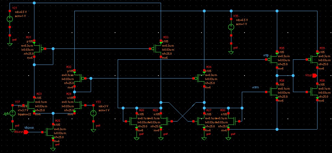
Figure 4: Voltage Comparator constructed in HSPICE
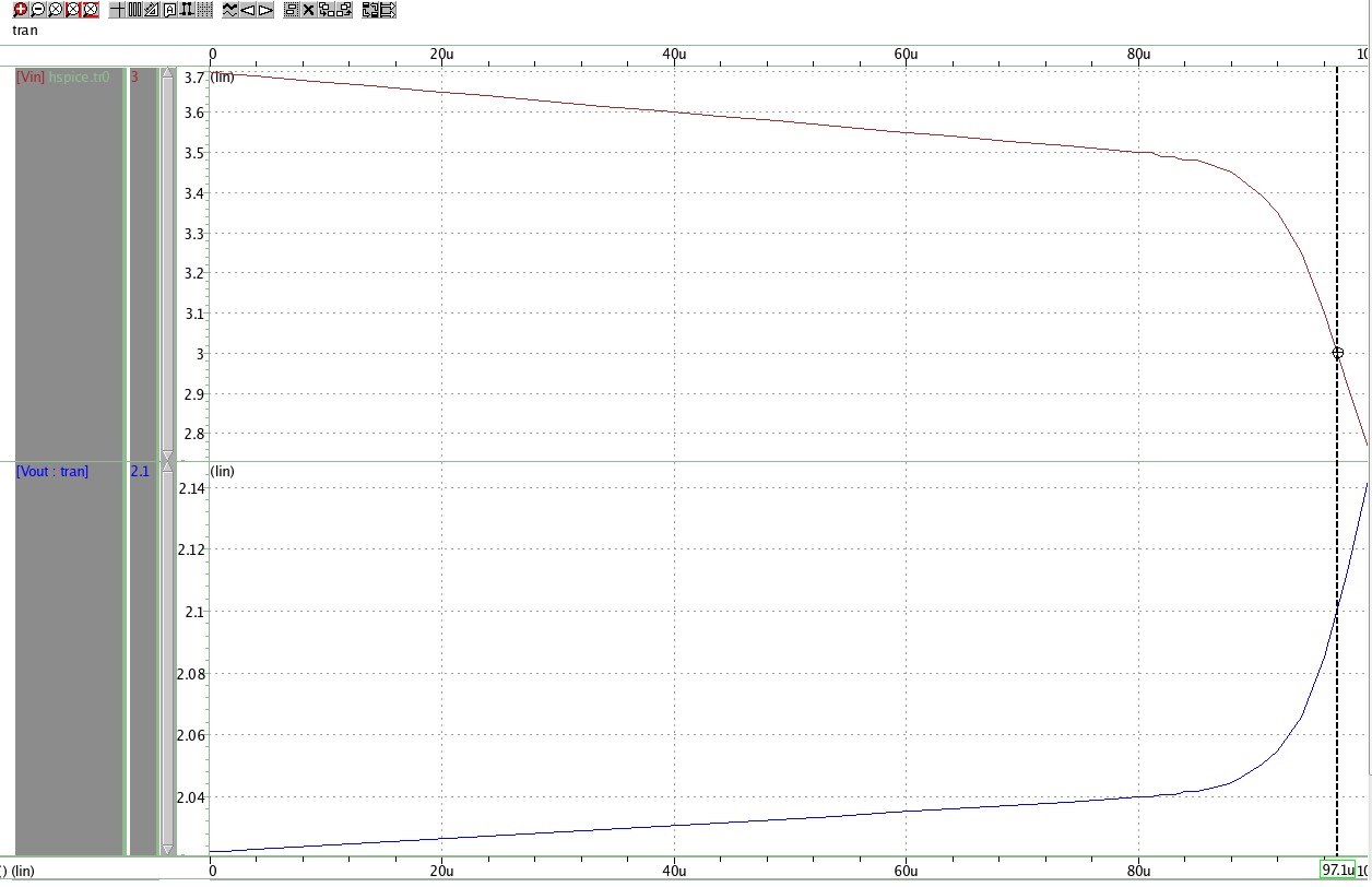
Figure 5: Transient Analysis of Voltage Comparator
After the comparator circuit was constructed in HSPICE and simulated, considerations were made for continuous battery sensing. The text was not used to construct this circuit, as its use case was a bit too specific to expect to find. This design used four stages of the voltage comparator circuit to create four different stages of battery charge indication. Aside from the four stages of comparators, no extra FETs were used. But a total of 12 resistors were added to the circuit, totalling 60 FETs and 12 resistors for this circuit. Its behavior is similar to the comparator circuit, but has several levels of voltage that would be used in the opposite manner. LEDs could be connected where the measurement pins were placed in the circuit, representing the charge level, but instead more would light up when the system reads a higher charge rather than the LEDs being an indicator of an emergency. The circuit is shown in Figure 6 and its behavior is shown in Figure 7.
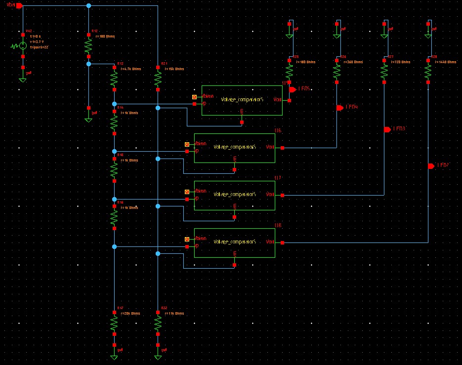
Figure 6: Continuous Indicator constructed in HSPICE
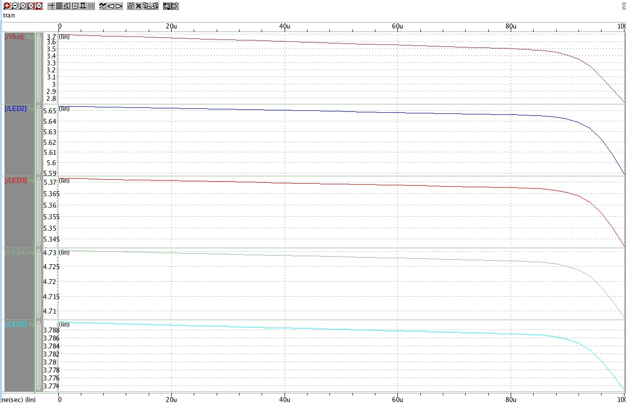
Figure 7: Transient Analysis of Continuous Indicator
The challenges that the team endured included creating the definite exponential decay of the lithium ion battery and a continuous reading of the % charge of the battery. A small portion of the project that gave the team a tough time was creating the exponential decay of the battery. At first, the group set a linear decay from 20% to 0%. But after some tampering around with the time values of the piecewise-linear voltage source, the error was resolved by increasing the time values little by little and decreased the voltages little by little, more like the exponential decay given in the specification sheet. This solution allowed the linear decay to transform into the desired exponential decay. Moreover, most of the group’s time went into making modifications to the voltage comparator so that it could work efficiently with the lithium ion battery. At first, it showed only the typical response of a comparator. In order to fix the error, an output buffer was connected to the voltage comparator so that the simulation displayed would show the battery discharging and the comparator’s response to the discharge.
Overall, the group learned how to build a lithium ion battery with a graphite anode, a voltage comparator, a continuous indicator, how to properly simulate all of them, and also more on how to troubleshoot HSPICE errors. This design project was an opportunity to demonstrate finesse in HSPICE, Simulation and Analysis Environment (SAE), and netlisting.